Not known Details About Countif Excel

By pressing ctrl+shift+facility, this will certainly determine and also return worth from several arrays, as opposed to just specific cells included in or increased by each other. Calculating the amount, item, or quotient of private cells is easy-- just utilize the =AMOUNT formula and go into the cells, worths, or series of cells you intend to execute that arithmetic on.

If you're aiming to find overall sales earnings from a number of offered units, as an example, the selection formula in Excel is perfect for you. Right here's just how you 'd do it: To start utilizing the selection formula, type "=AMOUNT," and also in parentheses, enter the first of 2 (or 3, or four) varieties of cells you would certainly like to multiply with each other.

This represents multiplication. Following this asterisk, enter your 2nd array of cells. You'll be multiplying this second variety of cells by the initial. Your progress in this formula should now resemble this: =AMOUNT(C 2: C 5 * D 2:D 5) Ready to press Enter? Not so quick ... Due to the fact that this formula is so challenging, Excel gets a various key-board command for varieties.

This will certainly acknowledge your formula as a variety, wrapping your formula in brace personalities and successfully returning your item of both varieties combined. In revenue computations, this can reduce down on your time and effort dramatically. See the final formula in the screenshot over. The MATTER formula in Excel is represented =COUNT(Start Cell: End Cell).

For instance, if there are eight cells with gone into values in between A 1 as well as A 10, =MATTER(A 1: A 10) will certainly return a value of 8. The MATTER formula in Excel is specifically helpful for big spreadsheets, wherein you want to see exactly how lots of cells contain actual entrances. Do not be deceived: This formula will not do any kind of mathematics on the values of the cells themselves.

The smart Trick of Interview Questions That Nobody is Talking About

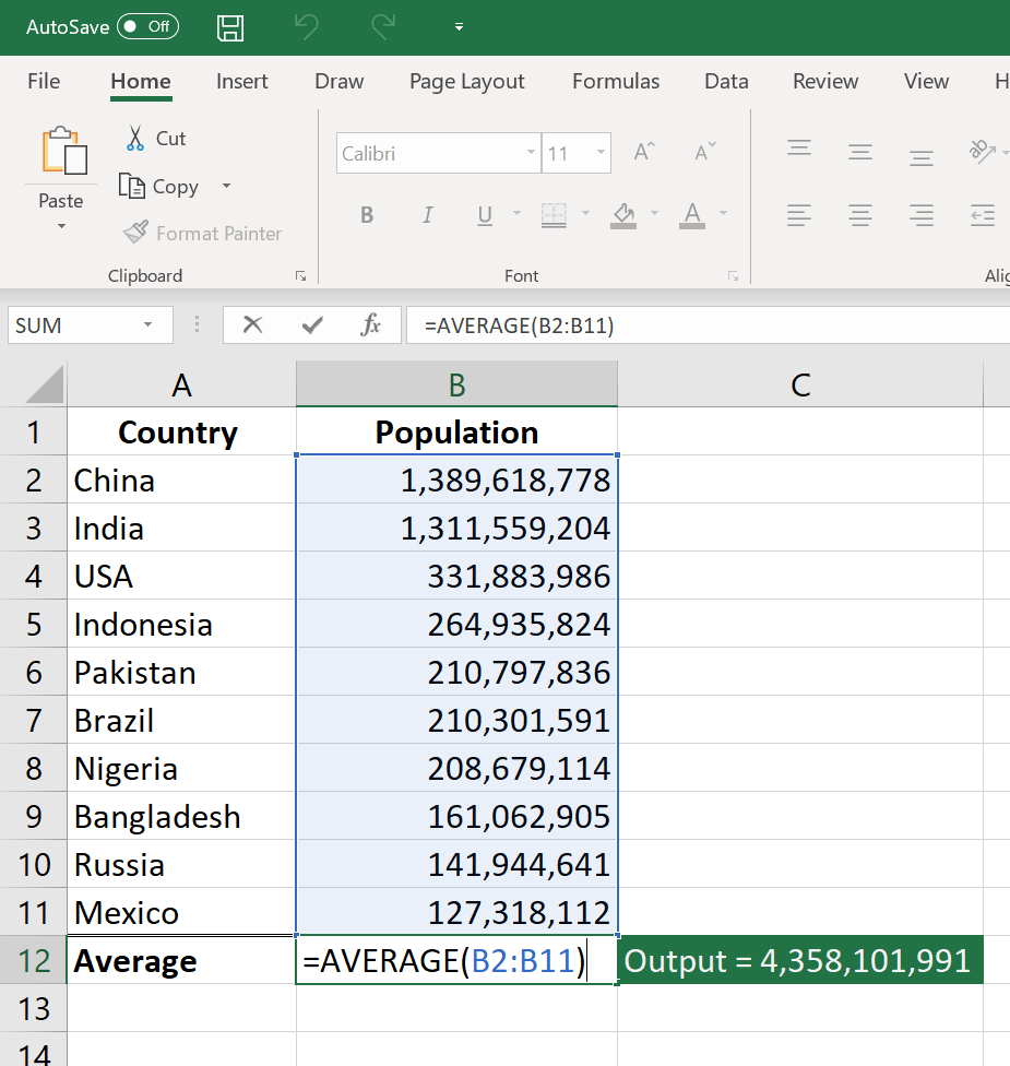
Utilizing the formula in bold above, you can conveniently run a matter of energetic cells in your spread sheet. The result will look a something similar to this: To do the average formula in Excel, go into the values, cells, or range of cells of which you're computing the average in the layout, =STANDARD(number 1, number 2, etc.) or =AVERAGE(Beginning Worth: End Value).

Locating the standard of a variety of cells in Excel maintains you from having to find specific sums and after that carrying out a separate department equation on your total. Making use of =AVERAGE as your first message entrance, you can let Excel do all the job for you. For recommendation, the average of a team of numbers amounts to the sum of those numbers, divided by the variety of things in that group.

This will return the sum of the worths within a desired series of cells that all satisfy one requirement. As an example, =SUMIF(C 3: C 12,"> 70,000") would return the amount of worths between cells C 3 and C 12 from just the cells that are above 70,000. Let's claim you wish to determine the revenue you generated from a checklist of leads that are connected with specific location codes, or determine the amount of particular workers' incomes-- yet only if they drop above a certain quantity.

With the SUMIF function, it doesn't need to be-- you can quickly add up the amount of cells that fulfill specific criteria, like in the wage instance above. The formula: =SUMIF(array, requirements, [sum_range] Array: The range that is being checked using your standards. Requirements: The standards that identify which cells in Criteria_range 1 will certainly be totaled [Sum_range]: An optional series of cells you're mosting likely to accumulate along with the first Array went into.

In the example listed below, we intended to determine the amount of the incomes that were above $70,000. The SUMIF function accumulated the dollar quantities that exceeded that number in the cells C 3 via C 12, with the formula =SUMIF(C 3: C 12,"> 70,000"). The TRIM formula in Excel is denoted =TRIM(message).

3 Simple Techniques For Excel Jobs

As an example, if A 2 consists of the name" Steve Peterson" with undesirable rooms prior to the initial name, =TRIM(A 2) would certainly return "Steve Peterson" without spaces in a new cell. Email and submit sharing are remarkable tools in today's office. That is, until among your coworkers sends you a worksheet with some actually fashionable spacing.

Instead of fastidiously getting rid of as well as including areas as needed, you can tidy up any type of irregular spacing using the TRIM function, which is used to remove extra rooms from information (with the exception of solitary spaces between words). The formula: =TRIM(text). Text: The message or cell where you desire to get rid of areas.

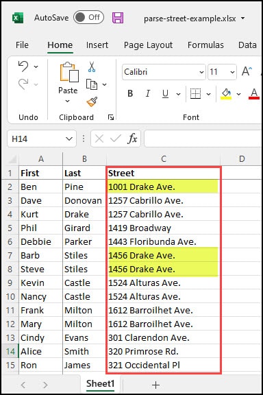
To do so, we entered =TRIM("A 2") into the Formula Bar, and also reproduced this for each and every name listed below it in a brand-new column beside the column with unwanted spaces. Below are some other Excel solutions you could locate beneficial as your information administration needs grow. Let's claim you have a line of message within a cell that you intend to damage down into a few different segments.

Objective: Made use of to remove the initial X numbers or characters in a cell. The formula: =LEFT(text, number_of_characters) Text: The string that you wish to extract from. Number_of_characters: The number of characters that you want to extract starting from the left-most personality. In the instance listed below, we got in =LEFT(A 2,4) right into cell B 2, and also duplicated it right into B 3: B 6.

Function: Made use of to extract personalities or numbers in the middle based on setting. The formula: =MID(message, start_position, number_of_characters) Text: The string that you wish to draw out from. Start_position: The placement in the string that you desire to begin drawing out from. For instance, the first position in the string is 1.

What Does Excel Formulas Do?

In this instance, we entered =MID(A 2,5,2) right into cell B 2, and also copied it into B 3: B 6. That permitted us to extract the 2 numbers beginning in the fifth position of the code. Purpose: Made use of to remove the last X numbers or characters in a cell. The formula: =RIGHT(text, number_of_characters) Text: The string that you want to draw out from.

formulas excel pdf 2013 excel formulas max excel formulas hide 0